Malaria Detection based on Blood Smear image with CNN and Tensorflow
Hello guys, welcome to my first article, so I recently finished a great course called Tensorflow In Practice by Deeplearning.ai on coursera that teaches how to use Tensorflow to build deep learning models.
So, in this article, I’d like to share about how I build a malaria detection model using Tensorflow from the preparation into prediction.
Before actually jump into the project, let me introduce you to some important component that I use for this article.
Tensorflow
TensorFlow is an end-to-end open-source platform for machine learning framework developed by Google’s Brain Team, it is being used in almost everywhere from industry to academia.
Why I use Tensorflow? Good question, well first because I’ve just finished a course that teaches me how to properly use it, second I think Tensorflow with it’s Keras API is the simplest way someone can build and train deep learning models and we’ll see it.
Google Colaboratory
Collaboratory or “Colab” for short is a free cloud-based Jupyter Notebook environment that allows us to train our machine learning and deep learning models on CPUs, GPUs, and TPUs.
So, if you like me that do not have access to unlimited computational power on our machines and think that buying GPU will result in a month of fasting I recommend using Colab for building deep learning models.
The Project
So, without more of boring chitchat let’s get started. Because this article is written in a Notebook you can open this article on Google Colab using this link. But, first read my article about prepare the colab notebook so that you can use the kaggle API.
Importing
First, we have to import all libraries that we need like the optimizer and all the layers to build a CNN model from tensorflow
Deep Learning
- Optimizer: RMSprop
- Layers : Convolutional, Max Pooling, Flatten and Dense
Visualization
- Matplotlib : for visualization in general
- PIL : Helper to show the image
Helper
- os : This module provides a portable way of using operating system dependent functionality.
- random : just like it’s name.
- shutil : The shutil module offers a number of high-level operations on files and collections of files. In particular, functions are provided which support file copying and removal.
- Pandas and Numpy : I don’t think I need to explain.
I won’t explain them, because it will need a whole page to explaining each one of them so maybe another time or you can click the link to learn more. For now, let’s focus on implementation.
## Helper
import os
import random
import shutil
import pandas as pd
import numpy as np

## Tensorflow
import tensorflow as tf
from tensorflow.keras.optimizers import RMSprop
from tensorflow.keras.preprocessing.image import ImageDataGenerator

## Visualization
from PIL import Image
import matplotlib.pyplot as plt
%matplotlib inline
Prepare the data
For the data I’ll use data from here.
If you already prepared colab based on the article before then you can just use kaggle API to download the dataset, to get the API command you can go to the dataset page and click on the vertical 3 dots button then copy api command just like the image below:
then just paste it into one of the code cell but add ‘!’ before the comman so that Colab know it is a command line not a python code, and because the downloaded data is zipped the we need to unzip it you can use python library called zipfile but I prefer to use the command line.
## Get the dataset Ready ##

# Install Kaggle and make directory for kaggle
!pip install -U -q kaggle && mkdir -p ~/.kaggle

# move json file from kaggle to the kaggle directory
!cp kaggle.json ~/.kaggle/

# Download the dataset
!kaggle datasets download -d iarunava/cell-images-for-detecting-malaria

# Unzip the dataset
!unzip -q cell-images-for-detecting-malaria -d data/
Warning: Your Kaggle API key is readable by other users on this system! To fix this, you can run 'chmod 600 /root/.kaggle/kaggle.json'
Downloading cell-images-for-detecting-malaria.zip to /content
 98% 665M/675M [00:15<00:00, 32.0MB/s]
100% 675M/675M [00:15<00:00, 44.7MB/s]
After running code above the you should see a new directory called data on colab files if not try click refresh button.
If you inspect the data directory then you can see that there’s subdirectory called cell_images and if you open it you can see that it’s already divided based on class Parasitized and Uninfected so we can use tensorflow ImageDataGenerator to automatically load the image and label it based on the name of the subdirectory in a given directory.
But there are no directory for test data so let’s make a new directory and take some iamge for test data
there also a duplicate cell_images directory so let’s remove it
shutil.rmtree('/content/data/cell_images/cell_images')
parasitized_dir = '/content/data/cell_images/Parasitized/'
uninfected_dir = '/content/data/cell_images/Uninfected/'
parasitized_dir_test = '/content/data/test/Parasitized/'
uninfected_dir_test = '/content/data/test/Uninfected/'

os.makedirs(parasitized_dir_test)
os.makedirs(uninfected_dir_test)
def split_test(test_size=0.2):
  classes = ['P','U']
  parasitized_files = os.listdir(parasitized_dir)
  uninfected_files = os.listdir(uninfected_dir)
  total_image = len(parasitized_files) + len(uninfected_files)
  for i in range(round(test_size*total_image)):
    clas = random.choice(classes)
    if clas == 'P':
      filename = random.choice(parasitized_files)
      PATH_SOURCE = parasitized_dir+filename
      PATH_DEST = parasitized_dir_test+filename
      shutil.move(PATH_SOURCE,PATH_DEST)
      parasitized_files.remove(filename)
    else:
      filename = random.choice(uninfected_files)
      PATH_SOURCE = uninfected_dir+filename
      PATH_DEST = uninfected_dir_test+filename
      shutil.move(PATH_SOURCE,PATH_DEST)
      uninfected_files.remove(filename)


split_test()
The sub-directory should be gone by now and there is new subdirectory name test.
Load The Image and Augmentation
Load Image
We’ll now use flow_from_dataframe method from ImageDataGenerator to load the image and feed it into our model by giving it metadata dataframe and specify the column for image name and label also the directory of all image.
Augmenting
While we load each of the image we will create the transformed version of the image.
Transforms include a range of operations from the field of image manipulation, such as shifts, flips, zooms, and much more. But, because because it’s a medical image and image of a blood smear I think the variation is not big so we will just zoom, flip it horizontally and vertically.
The intent is to expand the training dataset with new, plausible examples.
train_datagen = ImageDataGenerator(rescale=1/255,
                                   horizontal_flip=True,
                                   zoom_range=0.2,
                                   vertical_flip=True,
                                   validation_split=0.3) ## Image generator with augmentation

test_datagen = ImageDataGenerator(rescale=1/255)


TRAINING_DIR = "/content/data/cell_images"
TESTING_DIR = "/content/data/test"
train_generator=train_datagen.flow_from_directory(directory=TRAINING_DIR,
                                            subset="training",
                                            batch_size=32,
                                            seed=42,
                                            shuffle=True,
                                            class_mode="binary",
                                            target_size=(100,100))

validation_generator=train_datagen.flow_from_directory(directory=TRAINING_DIR,
                                            subset="validation",
                                            batch_size=32,
                                            seed=42,
                                            shuffle=True,
                                            class_mode="binary",
                                            target_size=(100,100))

test_generator = test_datagen.flow_from_directory(TESTING_DIR,
                                                  batch_size=32,
                                                  target_size=(100,100),
                                                  class_mode='binary')
Found 15433 images belonging to 2 classes.
Found 6614 images belonging to 2 classes.
Found 5511 images belonging to 2 classes.
We can see that there are:
- 15433 Image for training
- 6614 Image for validation
- 5511 Image for testing
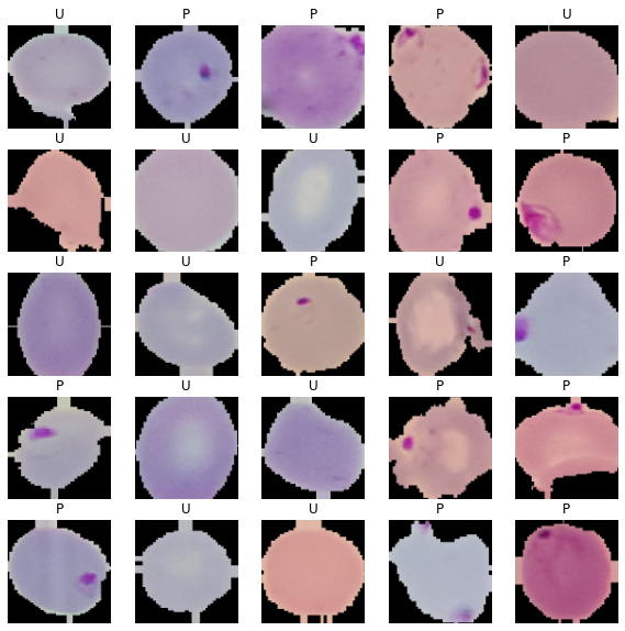
Let’s look at the image with our own eyes, and see whether we can differentiate between each class or not.
You also can see if the augmentation still make sense if not you can change it.
CLASS_NAMES = ['Parasitized','Uninfected']
def show_batch(image_batch, label_batch):
  plt.figure(figsize=(10,10))
  for n in range(25):
      ax = plt.subplot(5,5,n+1)
      plt.imshow(image_batch[n])
      plt.title(CLASS_NAMES[label_batch[n]==1][0].title())
      plt.axis('off')

image_batch, label_batch = next(train_generator)
show_batch(image_batch, label_batch)
/usr/local/lib/python3.6/dist-packages/ipykernel_launcher.py:7: DeprecationWarning: In future, it will be an error for 'np.bool_' scalars to be interpreted as an index
  import sys

You can see that it’s not hard to see the different with just our own eyes, so hopefully our model can get a good score.
Building the model
It’s a good practice for building a deep learning model is to first search a paper that try to solve similar problem and apply their architecture to your own problem.
So, I will use the architecture from this paper where they use CNN to detect malaria, you can click on the link if you want to read more about it, below are the architecture.
The Architectue
Here we gonna use the same architecture but for the regulazitation we will use BatchNormalization instead of Dropout. Given on this article by Harrison Jansma said that it’s better to use BatchNormalization on convolutional network than Dropout.
if you confuse on how to read the architecture below are a little description:
- Convolution 3 * 3 * 3@32: Convolution layer with kernel 3*3 and 32 Filters
- Max-pooling 2 * 2 / 2: max pooling layer with 2*2 pooling window and 2 pixel strides
- ReLU : Regular ReLU activation
- Fully Connected 1 * 1 * 64@64: Dense layer with 64 neurons
tf.keras.backend.clear_session()
model = tf.keras.models.Sequential([
    # 1st convolution
    tf.keras.layers.Conv2D(32, (3,3), activation='relu', input_shape=(100, 100, 3)),
    tf.keras.layers.BatchNormalization(),
    tf.keras.layers.MaxPooling2D(2, 2),
    # 2nd convolution
    tf.keras.layers.Conv2D(32, (3,3), activation='relu'),
    tf.keras.layers.BatchNormalization(),
    tf.keras.layers.MaxPooling2D(2,2),
    # 3rd convolution
    tf.keras.layers.Conv2D(64, (3,3), activation='relu'),
    tf.keras.layers.BatchNormalization(),
    tf.keras.layers.MaxPooling2D(2,2),
    # Flatten the results to feed into a DNN
    tf.keras.layers.Flatten(),
    # 64 neuron hidden layer
    tf.keras.layers.Dense(16, activation='relu'),
    # 1 output neuron with sigmoid activation function. because we only have 2 class
    tf.keras.layers.Dense(1, activation='sigmoid')
])


model.compile(optimizer=RMSprop(lr=1e-3), loss='binary_crossentropy', metrics=['accuracy'])
Training the model
We will train the model with 10 epoch but I also add callbacks to save our model everytime our validation accuracy increase and early stop if our validation loss is not decreasing for 3 epoch.
## Callbacks
os.makedirs('/content/checkpoint/',exist_ok=True)
checkpoint_filepath = '/content/checkpoint/' ##
model_checkpoint = tf.keras.callbacks.ModelCheckpoint(
    filepath=checkpoint_filepath,
    save_weights_only=True,
    monitor='val_accuracy',
    mode='max',
    save_best_only=True)

model_earlystop = tf.keras.callbacks.EarlyStopping(monitor='val_loss', patience=3)

history = model.fit(train_generator,
                    epochs=10,
                    verbose=1,
                    validation_data = validation_generator,
                    callbacks=[model_checkpoint,model_earlystop])
Epoch 1/10
483/483 [==============================] - 81s 167ms/step - loss: 0.4156 - accuracy: 0.7966 - val_loss: 0.6542 - val_accuracy: 0.6243
Epoch 2/10
483/483 [==============================] - 80s 165ms/step - loss: 0.2045 - accuracy: 0.9365 - val_loss: 0.2004 - val_accuracy: 0.9238
Epoch 3/10
483/483 [==============================] - 80s 165ms/step - loss: 0.1853 - accuracy: 0.9428 - val_loss: 0.2733 - val_accuracy: 0.9019
Epoch 4/10
483/483 [==============================] - 79s 163ms/step - loss: 0.1753 - accuracy: 0.9447 - val_loss: 0.2019 - val_accuracy: 0.9419
Epoch 5/10
483/483 [==============================] - 77s 159ms/step - loss: 0.1704 - accuracy: 0.9469 - val_loss: 0.2915 - val_accuracy: 0.8981
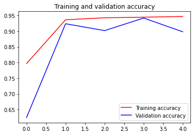
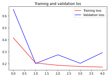
See, our training end at 5 epoch instead of 10 because the validation is not decreasing from epoch 2,
Let’s plot how our accuracy and loss progress over epochs
acc = history.history['accuracy']
val_acc = history.history['val_accuracy']
loss = history.history['loss']
val_loss = history.history['val_loss']

epochs = range(len(acc))

plt.plot(epochs, acc, 'r', label='Training accuracy')
plt.plot(epochs, val_acc, 'b', label='Validation accuracy')
plt.title('Training and validation accuracy')
plt.legend(loc=0)
plt.figure()

plt.show()


plt.plot(epochs, loss, 'r', label='Training loss')
plt.plot(epochs, val_loss, 'b', label='Validation loss')
plt.title('Training and validation los')
plt.legend(loc=0)
plt.figure()


plt.show()

<Figure size 432x288 with 0 Axes>

<Figure size 432x288 with 0 Axes>
We can see the training loss and accuracy is consistently decreasing while the validation is a little spiky but we can say that for sure given our training is ended prematurely with only 5 epoch.
You can try change the patience on EarlyEpoch to bigger value and see how the validation loss and accuracy goes for a longer period.
Evaluate using test data
Here we gonna evalute the model using test data that we already split before.
model.evaluate(test_generator)
173/173 [==============================] - 6s 37ms/step - loss: 0.2800 - accuracy: 0.8975


[0.2800314724445343, 0.8974777460098267]
We got 0.89 accuracy on the test data, I think it’s already good enough given we only train it with 5 epoch, try train for more epoch and see whether it actually increade the accuracy!
Sanity Check
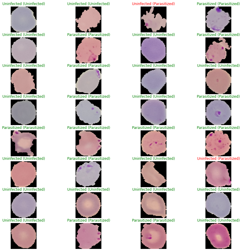
Even if I know the accuracy already good, I still want to inspect our model prediction in each picture and see the different between the image our model got right and the image our model got wrong.
image_batch, label_batch = next(test_generator)
preds = model.predict(image_batch)>0.5
plt.figure(figsize=(15,15))
for i in range(32):
  ax = plt.subplot(8,4,i+1)
  plt.imshow(image_batch[i])
  ax.set_title("{} ({})".format(CLASS_NAMES[int(preds[i])], CLASS_NAMES[int(label_batch[i])]),
                 color=("green" if int(preds[i])==int(label_batch[i].item()) else "red"))
  plt.axis('off')

We can see that from this batch we have 2 image that our model got wrong, one of the image is so distort and the parasite is on edge of the blood smear and the second on the second the parasite is spread around all area of blood smear so that different in color is not so big, I our model doesn’t generalize well in those kind of image.
What we can do is some type of preprocessing that make the different in color more clear and also add shifting the image to the augmentation.
END
So that’s it, how I build a model to detect malaria there are still things to explore on your own. I hope this article can give you a sense how you can build your own CNN using Tensorflow.
See you in next article!

